Many of the options are redundant to all plot types whereas others are unique. I will discuss them all below, but I won’t become repetitive. The time series description will be most in depth. Subsequent plot classes will benefit from redundant options and behaviour.

X-axis

The y-axis will be the selected climate variable, temperature or precipitation. For this reason there is only an x-axis choice, X-axis (time), at the top of the plot options panel when on the Time Series plot tab. Since these are time series plots, the x-axis is always time. The user may select month, year, or decade. This is a good place to point out the importance of thinking about what we want to graph. For example, if the user selects only January data across a number of years, it doesn’t make sense to use Month as the x-axis variable, unless they really want to see the vertical spread of all their years’ January values clustered at a single x-axis tick mark. But the app will allow the user to do this if so desired!

Grouping

Now things get more interesting. The grouping variable. This is a factor (categorical variable) with multiple levels. The text above the selection menu, Group/color by: suggests the use can color code data in a plot by different levels of a factor. This list populates with any factors in the user’s defined data subset which include at least two distinct levels (otherwise there is nothing to color differently). By default no grouping variable is selected. If one is chosen, color options will immediately appear lower in the plot options panel. They remain hidden if they are not applicable. Note that it is possible to select such a minimal amount of data that there will be no factors with multiple levels. In such a case the Group/color by: menu will not appear.

Faceting

To facet is to break out different classes of data into multiple panels in a plot. The Facet/panel by: title of this menu hints at this purpose. Like grouping, the faceting variable must be categorical with multiple levels present in the data. The default is no faceting and as with grouping, if no multi-level factors are present in the user’s data subset, this menu will not appear. All the same options available to group by are available to facet by, less any variable currently selected as a grouping variable (this last part is subject to change). As a result, an update to the Group/color by: by the user will force a reset/update to Facet/panel by: Also, if the data subset contains only one multi-level factor, both grouping and faceting options are available. However, in this special case, if that variable is selected for grouping, the faceting menu must vanish because no options remain.

Details

Some variables available to group or facet by include those available under X-axis (time). The user is prohibited from grouping or faceting by year as this often results in too many colors or panels, respectively. However, the user can certainly group or facet by month or decade. If one of these two is in use as the x-axis variable, it will not be available for grouping or faceting (this is subject to change).

Dependent on the X-axis (time),Group/color by:, andFacet/panel by:` selections, and the user-defined data subset, there may remain additional variables which would be pooled together in a graph such that they would not be uniquely identifiable. Say the data subset contains multiple levels of several variables. For example, three months, five models, and two locations. The user may elect to use years for the x-axis, group by model, and panel by location. This leaves three different months of data in the plot undistinguished from one another. The colors are for the different models. The side by side panels are for contrasting the two locations. Now there will be three points in the graph at each x-axis tick mark, and or lines for each. Just below the x-axis, grouping, and faceting menus text will appear to help the user keep track of any pooled variables.

Checkbox Options

Each plot type offers a number of additional options. The first few options, Title, Panel text, and Show CRU 3.2 are common available for all plots. When checked, the plot displays with a title, any in-panel text annotations (if applicable to the plot and/or data), and includes CRU data, respectively.

Next are the Show points, Jitter points, and Show lines checkboxes. Showing points and lines is clear. Jittering the point data is useful for when several points lie directly on top of one another given a discrete x-axis variable.

The Trend lines checkbox is distinct from the Show lines checkbox. The latter is for each observation and essentially connects points. The former shows a single line representing the mean of all the pooled data, or a set of differently colored lines in the case of grouping where each line is the average for a specific group.

Log transformations are also available for non-negative valued variables. A value of one is added prior to taking the log so as to avoid taking the log of zero or obtaining negative values.

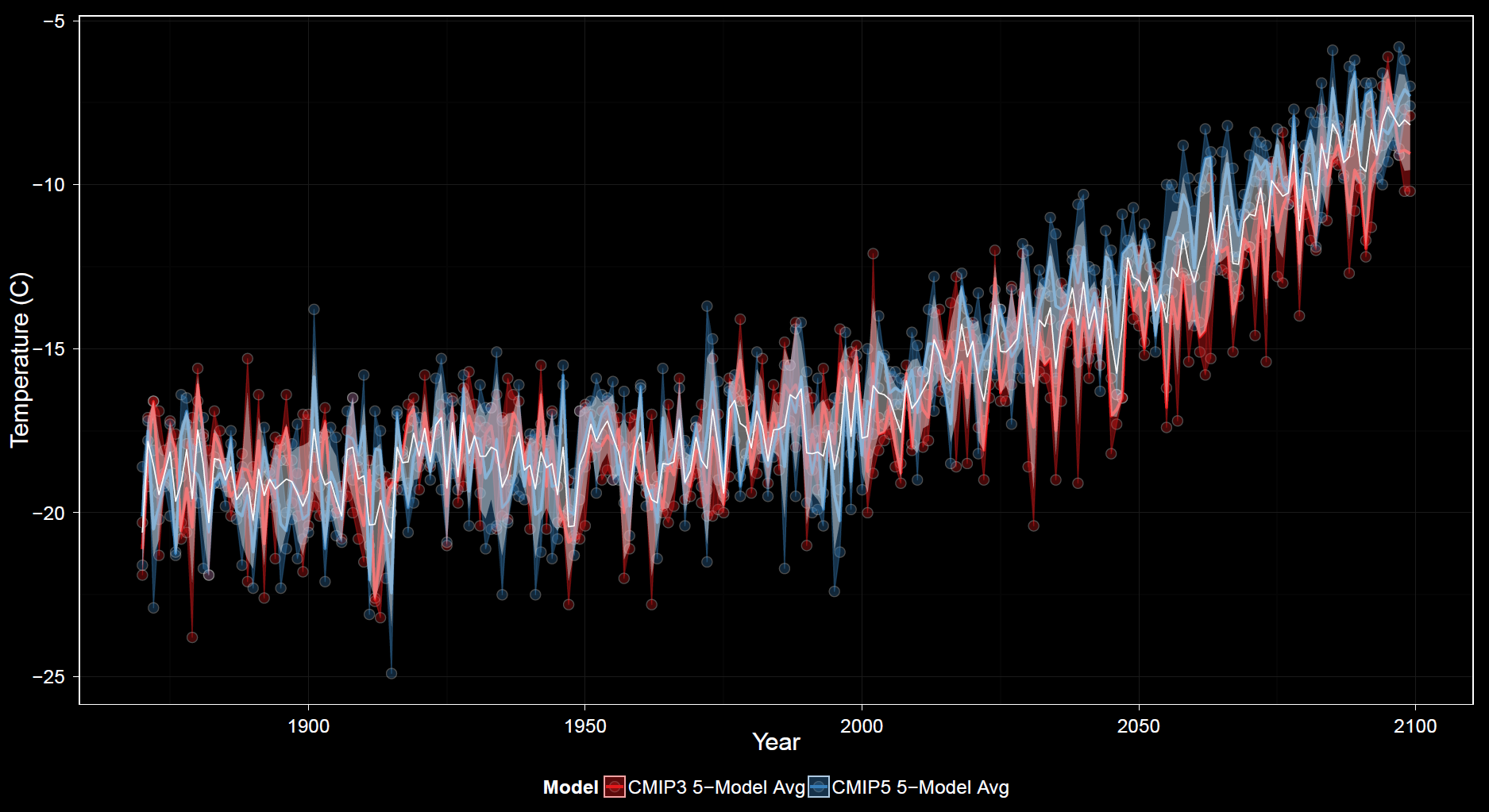
The Dark theme checkbox is unchecked by default. When checked the plot will take on a black background and previously black colors such as text or lines will switch to white.

There are also checkboxes showing the data range by group, Group range, and confidence bands around trend lines by group, Confidence band, but these are subject to change.

After all of these checkboxes, the user has some additional drop down menus. First are Transparency and Font size. Depending on user data selections, this may be all that appears. If a grouping variable is present, there will also be a Color palette menu. Color palette selections are grouped by type of color leveling subheadings: nominal, increasing, centered, and cyclic. Depending on characteristics of the grouping variable such as type of factor and number of levels, not all may be shown. If the grouping variable is nominal (unordered, e.g., Model) only this option is available. If the grouping variable has too many levels, only certain options will appear as well. With enough levels the color becomes restricted to evenly spaced values of a given color spectrum to try to maintain as much visual distinction as possible. My suggestion is that if this is a problem, you should use any of the plethora of other options available to distinguish so many factor levels.

When using a grouping variable, this is also the only time when the Legend positioning menu appears.

Special Case: Precipitation

Additional options are available when graphing precipitation time series because it has a real zero. We see precipitation as an amount. We cannot “add” temperatures together for instance. When precipitation is graphed, the user will see an additional Barplot checkbox. When making a time series of bars, the user may still overlay points, lines, and trend lines. A menu appears allowing the user to alternate between default horizontal and vertical bars. If grouping by a factor, the Barplot style menu appears to the right. The options are to Dodge (adjacent groupings), Stack (into a single bar), or Fill (show as relative proportions contributed by each group). When stacking or filling, it no longer makes sense to overlay points or lines because the scale has changes. Of course, the app will let the user do this is they really want to. But it will become apparent by the stretch of the graph axis that it is not very helpful to look at the data in this way. The app is very flexible. It will allow the user to plot many things which are clear and insightful, and many things which are not. Think before you plot.

Making and Remaking Graphs

To plot, press the Generate Plot button. To download a currently displayed plot, press the Download Plot button. It’s that simple. To make changes to a plot, you can alter values in the plot options panel at any time. Due to natural dependencies, changing some options will force resets and updates of other options. Note that if you reopen the data selections menu and change anything you will be required to restart by completing a new data subset and making a new plot.