The rtrek package includes some Star Trek datasets, but
much more data is available outside the package. You can access other
Star Trek data through various APIs.
Technically, there is only one formal API: the Star Trek API (STAPI).
rtrek has functions to assist with making calls to this API
in order to access specific data. This is the focus of this
vignette.
rtrek also interfaces with and extracts information from
the Memory
Alpha and Memory Beta
websites. Neither of these sites actually expose an API, but functions
in rtrek with querying these websites in an API-like
manner. See the respective vignettes for details.
Accessing information from STAPI is covered to some degree in the package introduction vignette. There is some duplication here, followed by additional examples.
Star Trek API
The Star Trek API (STAPI) is a particularly useful data source.
Keep in mind that STAPI focuses more on providing real world data associated with Star Trek (e.g., when did episode X first air on television?) than on fictional universe data, but it contains both and the database holdings will grow with time.
To use the words of the developers, the STAPI is
the first public Star Trek API, accessible via REST and SOAP. It’s an open source project, that anyone can contribute to.
The API is highly functional. Please do not abuse the API with
constant requests. Their pages suggest no more than one request per
second, but I would suggest ten seconds between successive requests. The
default anti-DDOS measures in rtrek limit requests to one
per second. You can update this global rtrek setting with
options(), e.g. options(rtrek_antidos = 10)
for a minimum ten second wait between API calls to be an even better
neighbor. rtrek will not permit faster requests. If set
below one second, the option is ignored and a warning thrown when making
any API call.
STAPI entities
There a many fields, or entities, available in the API. The available IDs can be found in this table:
stapiEntities
#> # A tibble: 40 × 4
#>    id                 class   ncol colnames
#>    <chr>              <chr>  <int> <named list>
#>  1 animal             tbl_df     7 <chr [7]>
#>  2 astronomicalObject tbl_df     5 <chr [5]>
#>  3 book               tbl_df    24 <chr [24]>
#>  4 bookCollection     tbl_df    10 <chr [10]>
#>  5 bookSeries         tbl_df    11 <chr [11]>
#>  6 character          tbl_df    24 <chr [24]>
#>  7 comicCollection    tbl_df    14 <chr [14]>
#>  8 comics             tbl_df    15 <chr [15]>
#>  9 comicSeries        tbl_df    15 <chr [15]>
#> 10 comicStrip         tbl_df    12 <chr [12]>
#> # ℹ 30 more rows
These ID values are passed to stapi() to perform a
search using the API. The other columns provide some information about
the object returned from a search. All entity searches return tibble
data frames. You can inspect or unnest the column names of each table
returned from every available entity search so you can see beforehand
what variables are associated with each entity.
Accessing the API
Using stapi should be thought of as a three part
process:
- Determine how many pages of results exist for a particular entity search.
- Only after taking care to do the previous step, perform the search to return search results.
- If satellite data is needed on a unique observation in the search
results, call
stapi()one more time referencing the specific observation.
To determine how many pages of results exist for a given search, set
page_count = TRUE. The impact on the API will be equivalent
to only searching a single page of results. One page contains metadata
including the total number of pages. Nothing is returned in this “safe
mode”, but the total number of search results available is printed to
the console.
Searching movies only returns one page of results. However, there are a lot of characters in the Star Trek universe. Check the total pages available for character search.
stapi("character", page_count = TRUE)
#> Total pages to retrieve all results: 76
And that is with 100 results per page!
The default page = 1 only returns the first page.
page can be a vector, e.g. page = 1:62.
Results from multi-page searches are automatically combined into a
single, constant data frame output. For the second call to
stapi(), return only page two here, which contains the
character, Q (currently, pending future character database updates that
may shift the indexing). In case that does change and Q is not always
near the top of page two of the search results, the example further
below hard-codes his unique/universal ID.
library(dplyr)
stapi("character", page = 1) %>% select(uid, name)
#> # A tibble: 100 × 2
#>    uid            name
#>    <chr>          <chr>
#>  1 CHMA0000215045 0413 Theta
#>  2 CHMA0000174718 0718
#>  3 CHMA0000283851 10111
#>  4 CHMA0000278055 335
#>  5 CHMA0000282741 355
#>  6 CHMA0000026532 A'trom
#>  7 CHMA0000280385 A. Armaganian
#>  8 CHMA0000226457 A. Baiers
#>  9 CHMA0000232390 A. Baiers
#> 10 CHMA0000068580 A. Banda
#> # ℹ 90 more rows
Character tables can be sparse. There are a lot of variables, many of which will contain missing data for rare, esoteric characters. Even for more popular characters about whom much more universe lore has been uncovered, it still takes dedicated nerds to enter all the data in a database.
When a dataset contains a uid column, this can be used
subsequently to extract a satellite dataset about that particular
observation that was returned in the original search. First you used
safe mode, then search mode, and now switch from search mode to
extraction mode to obtain data about Q, specifically. All that is
required to do this is pass Q’s uid to stapi()
and call the function one last time. When uid is no longer
NULL, stapi() knows not to bother with a
search and makes a different type of API call requesting information
about the uniquely identified entry.
Q <- "CHMA0000025118"
Q <- stapi("character", uid = Q)

q_eps <- Q$episodes %>% select(uid, title, stardateFrom, stardateTo)
q_eps
#>               uid                 title stardateFrom stardateTo
#> 1  EPMA0000259941               Veritas           NA         NA
#> 2  EPMA0000000651              Tapestry           NA         NA
#> 3  EPMA0000000500            Hide And Q      41590.5    41590.5
#> 4  EPMA0000277408        The Star Gazer           NA         NA
#> 5  EPMA0000280052              Farewell           NA         NA
#> 6  EPMA0000279099            Two of One           NA         NA
#> 7  EPMA0000278606               Watcher           NA         NA
#> 8  EPMA0000001510    The Q and the Grey      50384.2    50392.7
#> 9  EPMA0000001413                True Q      46192.3    46192.3
#> 10 EPMA0000000845                Q-Less      46531.2    46531.2
#> 11 EPMA0000001329                 Q Who      42761.3    42761.3
#> 12 EPMA0000278900    Fly Me to the Moon           NA         NA
#> 13 EPMA0000000483 Encounter at Farpoint      41153.7    41153.7
#> 14 EPMA0000001458    All Good Things...      47988.0    47988.0
#> 15 EPMA0000162588            Death Wish      49301.2    49301.2
#> 16 EPMA0000289337   The Last Generation           NA         NA
#> 17 EPMA0000001347                Deja Q      43539.1    43539.1
#> 18 EPMA0000277535               Penance           NA         NA
#> 19 EPMA0000278226          Assimilation           NA         NA
#> 20 EPMA0000279450                 Mercy           NA         NA
#> 21 EPMA0000001619                    Q2      54704.5    54704.5
#> 22 EPMA0000001377                  Qpid      44741.9    44741.9
The data returned on Q is actually a large list, including multiple data frames. For simplicity only a piece of it is shown above.
Find out which TNG characters other than Q appear in both the
Encounter at Farpoint series premier and later in the All
Good Things… series finale. To do this, usestapi() to
extract data from other endpoints by following a breadcrumb trail of
uid values.
Engage.
eps <- c("Encounter at Farpoint", "All Good Things...")
q_eps <- filter(q_eps, title %in% eps)
q_eps
#>              uid                 title stardateFrom stardateTo
#> 1 EPMA0000000483 Encounter at Farpoint      41153.7    41153.7
#> 2 EPMA0000001458    All Good Things...      47988.0    47988.0
eaf <- stapi("episode", uid = q_eps$uid[q_eps$title == eps[1]])
agt <- stapi("episode", uid = q_eps$uid[q_eps$title == eps[2]])
characters <- setdiff(intersect(eaf$characters$name, agt$characters$name), "Q")
characters
#> [1] "Data"             "Worf"             "Geordi La Forge"  "Deanna Troi"
#> [5] "William T. Riker" "Natasha Yar"      "Beverly Crusher"  "Jean-Luc Picard"
#> [9] "Miles O'Brien"
This returns key crew members who remained a part of the show from
beginning to end, disregarding any interim absences. Below, inspect how
many episodes each character appeared in. uid is again
needed, this time for each character.
Note that this requires making one API call for each character. The
anti-DOS measures in rtrek will force a one-second minimum
wait between each call in the event that the individual calls actually
return results faster than this, so the code below will take at least
seven seconds to complete.
Add a fun Star Trek-themed plot? Make it so.
characters <- eaf$characters %>% select(uid, name) %>% filter(name %in% characters)
characters
#>              uid             name
#> 1 CHMA0000261620             Data
#> 2 CHMA0000123141             Worf
#> 3 CHMA0000132570  Geordi La Forge
#> 4 CHMA0000123101      Deanna Troi
#> 5 CHMA0000123073 William T. Riker
#> 6 CHMA0000278224      Natasha Yar
#> 7 CHMA0000123143  Beverly Crusher
#> 8 CHMA0000289509  Jean-Luc Picard
#> 9 CHMA0000278225    Miles O'Brien
eps_count <- sapply(characters$uid, function(i){
  stapi("character", uid = i)$episodes$series |>
     summarize(sum(title == "Star Trek: The Next Generation")) |>
    unlist()
})
eps_count <- select(characters, name) |> mutate(n = eps_count)

library(ggplot2)
library(showtext)
font_add("StarNext", system.file(paste0("fonts/StarNext.ttf"), package = "trekfont"))
showtext_auto()

uniforms <- c("#5B1414", "#AD722C", "#1A6384")[c(3, 1, 2, 2, 2, 2, 2, 1, 3)]
eb <- element_blank()

ggplot(eps_count, aes(factor(name, levels = name[order(n)]), n)) +
  geom_col(fill = uniforms, color = "gray20") + coord_flip() +
  theme_minimal(base_size = 22) +
  theme(plot.title = element_text(family = "StarNext"), line = eb, axis.text.x = eb) +
  scale_x_discrete(expand = c(0, 0)) + scale_y_continuous(expand = c(0, 0)) +
  labs(x = NULL, y = NULL, title = "TNG EPISODE APPEARANCES") +
  geom_text(aes(label = n), color = "white", size = 8, hjust = 1.5)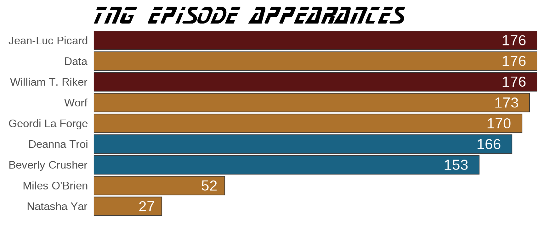
This looks as expected. Inspect the structure of the list objects
returned by stapi() to become more familiar with what kind
of information is available.
Minor weirdness
Sometimes you may receive errors when trying filter rows for one of
the data frames while certain problematic columns are still selected.
This is likely because the data frame contains a nested data frame, but
one which is not nested in the typical way (e.g.,
tidyr::unnest() will also fail to resolve the issue).
In the code immediately above, this occurs with the
series data frame, which is why the episodes
parent data frame is subset using $series before calling
dplyr::summarise().