These examples explore the word counts of published Star Trek novels
from 1967 through 2017 based on the stBooks dataset.
First, load packages to assist with data manipulation and plotting.
library(dplyr)
library(lubridate)
library(ggplot2)
library(ggrepel)
library(gridExtra)
library(rtrek) # use >= v0.2.1 for more accurate word count data
Look for trends in word count through time for select series: The
Next Generation, Deep Space Nine, and Voyager. Mutating the
date and nword columns facilitates a better
plot. Retain outliers in general, but drop any titles containing the
word “Omnibus” because these are known to be larger books containing
multiple individual novels. Inspect the data.
keep_series <- c("TNG", "DS9", "VOY")
x <- mutate(stBooks, date = decimal_date(as.Date(date)), nword = nword / 1000) %>%
  filter(series %in% keep_series & !grepl("Omnibus", title))

arrange(x, nword)
#> # A tibble: 266 × 11
#>    title   author  date publisher identifier series subseries nchap nword  nchar
#>    <chr>   <chr>  <dbl> <chr>     <chr>      <chr>  <chr>     <int> <dbl>  <int>
#>  1 Slings… Terri… 2008. Simon an… 1416550240 TNG    NA            8  10.7  63356
#>  2 Slings… Keith… 2008. Simon an… 978141655… TNG    NA           11  18.9 112768
#>  3 First … John … 1997. Pocket B… 978074345… TNG    NA           13  23.6 137531
#>  4 Slings… Willi… 2008. Simon an… 1416550224 TNG    NA            8  23.8 140719
#>  5 Typhon… Chris… 2012. Gallery … 978145165… TNG    Typhon P…    14  25.3 149530
#>  6 Lust's… Paula… 2015. Pocket B… 978147677… DS9    NA           16  25.5 188622
#>  7 Slings… Rober… 2008. Simon an… 978141655… TNG    NA            7  25.8 153414
#>  8 Q are … Rudy … 2015. Pocket B… 978147677… TNG    NA           10  27.2 192705
#>  9 Slings… J. St… 2008. Pocket B… 978141655… TNG    NA           12  27.6 159115
#> 10 The St… James… 2013. Pocket B… 978145169… TNG    NA            5  29.2 212328
#> # ℹ 256 more rows
#> # ℹ 1 more variable: dedication <chr>
Create a plot, separating each series in a different panel rather than using color to differentiate them.
clrs <- c("cornflowerblue", "orange", "purple")
ggplot(x, aes(date, nword, color = series, fill = series)) +
  geom_point(color = "black", shape = 21, size = 3) +
  geom_smooth(method = "lm", se = FALSE) +
  labs(title = "Star Trek novel word count", subtitle = "By publication date and selected series",
       x = "Publication date", y = "Word count (Thousand words)") +
  theme_minimal() + scale_color_manual(values = clrs) + scale_fill_manual(values = clrs) +
  scale_x_continuous(breaks = seq(1987, 2018, by = 3) + 0.5, labels = seq(1987, 2018, by = 3))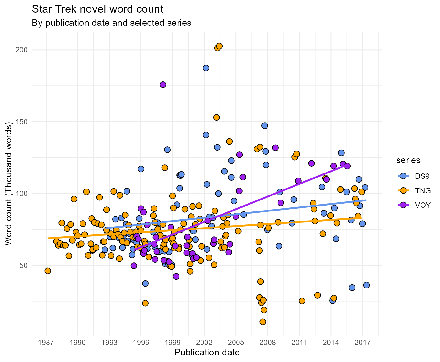
Look at the marginal change through time in average word count (pool all three series) with a simple linear model.
summary(lm(nword ~ date, data = x))
#>
#> Call:
#> lm(formula = nword ~ date, data = x)
#>
#> Residuals:
#>     Min      1Q  Median      3Q     Max
#> -73.630 -13.805  -3.222  10.338 121.988
#>
#> Coefficients:
#>               Estimate Std. Error t value Pr(>|t|)
#> (Intercept) -1705.3048   446.1422  -3.822 0.000165 ***
#> date            0.8912     0.2229   3.998  8.3e-05 ***
#> ---
#> Signif. codes:  0 '***' 0.001 '**' 0.01 '*' 0.05 '.' 0.1 ' ' 1
#>
#> Residual standard error: 27.17 on 264 degrees of freedom
#> Multiple R-squared:  0.05709,    Adjusted R-squared:  0.05352
#> F-statistic: 15.98 on 1 and 264 DF,  p-value: 8.298e-05
There is about a 40% increase in average word count per novel across the three series from the the first TNG novel in 1987 through 2017. In the case of the Voyager novels, however, the average word count approximately doubles and does so over a short production run. It is worth noting that as word count has trended upward noticeably, novels from these series have also been published less frequently. If you have read many of these book in paperback form, both the oldest and the more recent ones, this should not be a surprising result. Many of the newer releases have notably more pages and smaller font than the novels from the earlier years.
In this next example, consider all books from all series available in
stBooks, with the exception of Omnibus editions and those
falling into the reference category. This example looks at cumulative
total word count over time for all the selected books. For plot labeling
purposes, this time divide the word count by one million.
x <- mutate(stBooks, date = decimal_date(as.Date(date)), nword = nword / 1e6) %>%
  filter(series != "REF" & !grepl("Omnibus", title)) %>%
  arrange(date) %>%
  mutate(total_words = cumsum(nword))

x
#> # A tibble: 732 × 12
#>    title  author  date publisher identifier series subseries nchap  nword  nchar
#>    <chr>  <chr>  <dbl> <chr>     <chr>      <chr>  <chr>     <int>  <dbl>  <int>
#>  1 Banta… James… 1967  Amereon … 978084880… TOS    NA           NA 0.0411 235524
#>  2 Banta… James… 1968. Amereon … 978084880… TOS    NA           NA 0.0405 232094
#>  3 Banta… James… 1969. Bantam B… 978055312… TOS    NA           NA 0.0389 224369
#>  4 Banta… James… 1970. Bantam B… 978055310… TOS    NA            9 0.0361 207001
#>  5 Banta… James… 1971. Bantam B… 978055312… TOS    NA           NA 0.0416 239859
#>  6 Banta… James… 1972. Bantam B… 978055314… TOS    NA           NA 0.0430 247985
#>  7 Banta… James… 1972. Bantam B… 978055313… TOS    NA           NA 0.0428 248923
#>  8 Banta… James… 1972. Bantam B… 978055313… TOS    NA           NA 0.0464 268309
#>  9 Banta… James… 1973. Bantam B… 978055312… TOS    NA           NA 0.0533 307648
#> 10 Banta… James… 1974. Bantam B… 978055312… TOS    NA           NA 0.0533 314575
#> # ℹ 722 more rows
#> # ℹ 2 more variables: dedication <chr>, total_words <dbl>
The plot will be labeled with series abbreviations, so a key is needed for clarity. In order to label points on the plot marking the onset of a new novel series, take the first entry in the data frame for each series. A bit of theme customization is required for the table grid object that will display the key as an inset figure.
tab_theme <- gridExtra::ttheme_default(
  core = list(fg_params = list(cex = 0.5), padding = unit(c(2, 2), "mm")),
  colhead = list(fg_params = list(cex = 0.5)))

series <- group_by(x, series) %>% slice(1) %>% ungroup() %>%
  inner_join(stSeries, by = c("series" = "abb")) %>%
  select(series, id, date, total_words)

series
#> # A tibble: 20 × 4
#>    series id                                        date total_words
#>    <chr>  <chr>                                    <dbl>       <dbl>
#>  1 AV     Abramsverse                              2009.     41.4
#>  2 CT     Tales from the Captain's Table Anthology 1998.     17.4
#>  3 DS9    Deep Space Nine                          1993.      8.97
#>  4 DSC    Discovery                                2018.     52.1
#>  5 ENT    Enterprise                               2002.     24.5
#>  6 KE     Klingon Empire                           2004.     30.1
#>  7 MISC   Miscellaneous                            1995.     11.7
#>  8 NF     New Frontier                             1997.     15.7
#>  9 SCE    Starfleet Corps of Engineers             2001.     22.2
#> 10 SGZ    Stargazer                                2002.     25.6
#> 11 SKR    Seekers                                  2015.     48.1
#> 12 SNW    Strange New Worlds Anthology             1998.     17.5
#> 13 ST     All-Series/Crossover                     2000.     20.6
#> 14 SV     Shatnerverse                             1998.     17.2
#> 15 TLE    The Lost Era                             2004.     28.5
#> 16 TNG    The Next Generation                      1988.      4.01
#> 17 TOS    The Original Series                      1967       0.0411
#> 18 TTN    Titan                                    2005.     34.0
#> 19 VAN    Vanguard                                 2006.     34.7
#> 20 VOY    Voyager                                  1996.     13.2

key <- bind_rows(series, tibble(series = "YA-", id = "Young adult books")) %>%
  mutate(id = gsub(" Anthology", "", id)) %>%
  select(1:2) %>%
  setNames(c("Label", "Onset of book series")) %>%
  tableGrob(rows = NULL, theme = tab_theme)
Finally, create the plot.
brks <- c(1967, seq(1970, 2015, by = 5), 2018)

ggplot(x, aes(date, total_words)) +
  geom_step(size = 1, color = "gray30") +
  geom_point(data = series, shape = 21, fill = "#FF3030", size = 3) +
  geom_label_repel(data = series, aes(label = series), color = "white", fill = "#FF3030CC",
                   segment.color = "black", fontface = "bold", label.size = NA) +
  labs(title = "Star Trek novel cumulative word count",
       subtitle = "By publication date, excluding reference and omnibus titles",
       x = "Publication date",
       y = "Cumulative word count (Million words)") +
  theme_minimal() +
  scale_x_continuous(expand = c(0, 0), breaks = brks + 0.5, labels = brks) +
  scale_y_continuous(expand = c(0, 0)) +
  coord_cartesian(xlim = c(1966.5, 2019)) +
  annotation_custom(key, xmin = 2007, ymax = 35)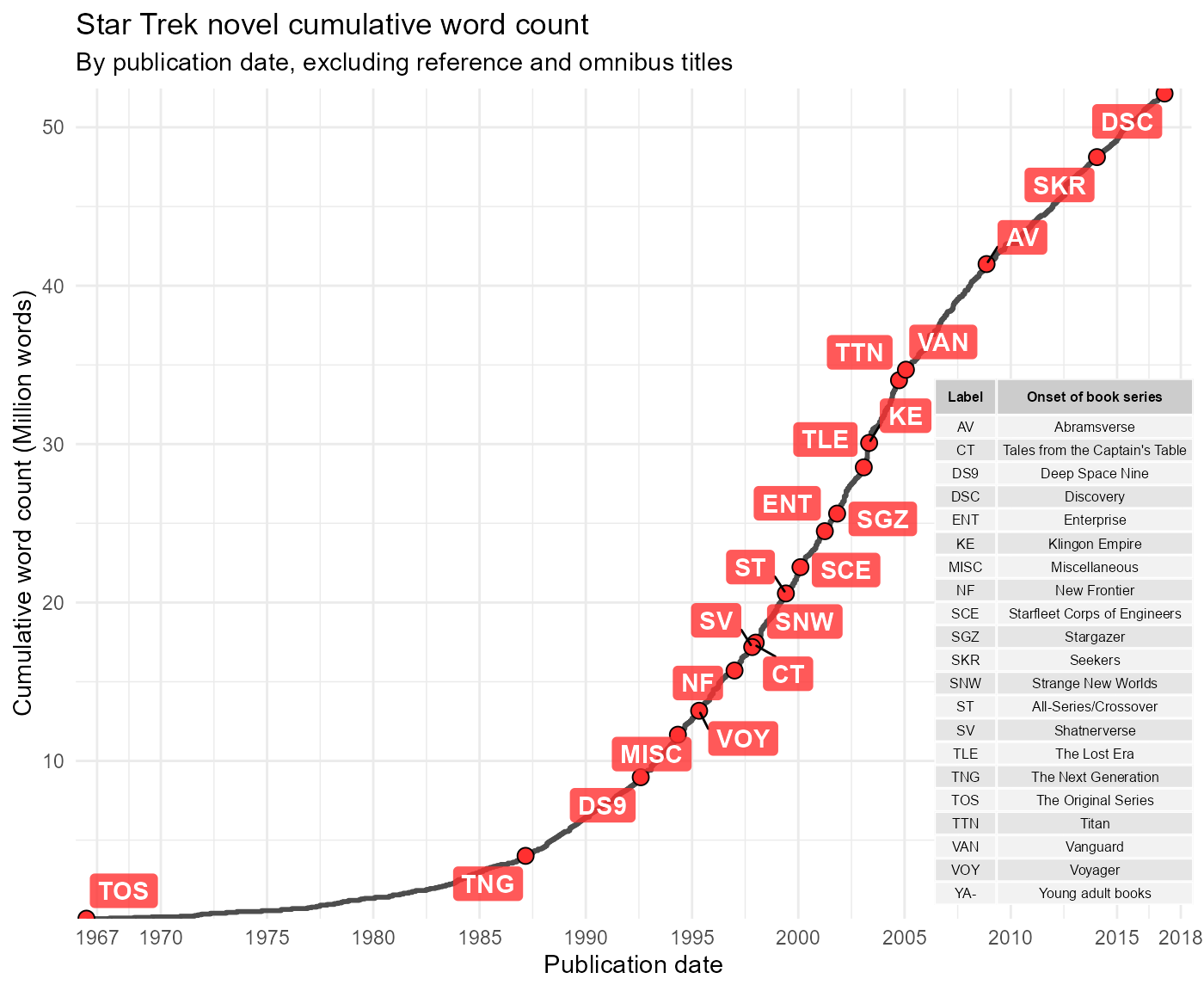
The golden age of licensed Star Trek novel publishing is clear. The 1990s and 2000s saw the creation of many new series as well of regular publication of new novels from existing ones. The current trajectory appears similar to the early 1990s, at least in terms of total words written. Data up to date only through 2017.