Importing transcript data
A curated data frame of metadata and text variables derived from
episode and movie transcripts can be downloaded with
st_transcripts(). The format is one episode per row. There
are metadata columns and a list column of nested text variables.
library(dplyr)
library(tidyr)
library(ggplot2)
library(ggrepel)

(scriptData <- st_transcripts())
#> # A tibble: 726 × 10
#>    format  series season number title    production airdate url   url2  text
#>    <chr>   <chr>   <int>  <int> <chr>         <int> <chr>   <chr> <chr> <list>
#>  1 episode TOS         1      0 The Cage          1 NA      http… http… <tibble>
#>  2 episode TOS         1      1 The Man…          6 1966-0… http… http… <tibble>
#>  3 episode TOS         1      2 Charlie…          8 1966-0… http… http… <tibble>
#>  4 episode TOS         1      3 Where N…          2 1966-0… http… http… <tibble>
#>  5 episode TOS         1      4 The Nak…          7 1966-0… http… http… <tibble>
#>  6 episode TOS         1      5 The Ene…          5 1966-1… http… http… <tibble>
#>  7 episode TOS         1      6 Mudd's …          4 1966-1… http… http… <tibble>
#>  8 episode TOS         1      7 What ar…         10 1966-1… http… http… <tibble>
#>  9 episode TOS         1      8 Miri             12 1966-1… http… http… <tibble>
#> 10 episode TOS         1      9 Dagger …         11 1966-1… http… http… <tibble>
#> # ℹ 716 more rows

scriptData$text[[81]]
#> # A tibble: 816 × 6
#>    line_number perspective                   setting description character line
#>          <int> <chr>                         <chr>   <chr>       <chr>     <chr>
#>  1          NA NA                            "Fade … NA          NA        NA
#>  2           1 Ext. Space - starship (optic… "The u… NA          Picard V… Capt…
#>  3           2 Other introductory angles (o… "On th… NA          Picard V… My o…
#>  4           3 Int. Engine room              "Huge,… Continuing  Picard V… ... …
#>  5           4 Closer on vessel diagram      "Showi… NA          Picard V… I am…
#>  6          NA Int. Lounge deck              "With … NA          NA        NA
#>  7           5 Continued                      NA     Continuing  Picard V… ... …
#>  8           6 Int. Bridge - wide angle      "Picar… Continuing  Picard V… ... …
#>  9           7 Angle emphasizing picard and… "As pi… NA          Picard    You …
#> 10           8 Angle emphasizing picard and…  NA     NA          Data      Diff…
#> # ℹ 806 more rows
Basic TNG summary
Consider TNG episodes. A rough estimate of the relative amount of speaking parts can be obtained by counting up the lines for each character. A better measure would be an estimate of word count taken from each spoken line. Calculate these statistics by season and episode as well as character.
Also remove unneeded columns. As is common in text analysis, even a
clean dataset may need further preparation for a specific task. In this
case it is important to strip references to things such as voice over
(V.o.) from the character column.
pat <- "('s\\s|\\s\\(|\\sV\\.).*"
x <- filter(scriptData, format == "episode" & series == "TNG") %>%
  unnest(text) %>%
  select(season, title, character, line) %>%
  mutate(character = gsub(pat, "", character)) %>%
  group_by(season, title, character) %>%
  summarize(lines = n(), words = length(unlist(strsplit(line, " "))))

x
#> # A tibble: 2,858 × 5
#> # Groups:   season, title [176]
#>    season title    character        lines words
#>     <int> <chr>    <chr>            <int> <int>
#>  1      1 11001001 Ad Libbed Voices     1    14
#>  2      1 11001001 Bass                 4    16
#>  3      1 11001001 Beverly              7   169
#>  4      1 11001001 Bynar One Zero       1     5
#>  5      1 11001001 Bynar Zero One       1     9
#>  6      1 11001001 Computer            11    96
#>  7      1 11001001 Computer Voice      14   129
#>  8      1 11001001 Data                31   361
#>  9      1 11001001 Drummer              2    22
#> 10      1 11001001 Geordi              23   166
#> # ℹ 2,848 more rows
Another limitation of using lines is that they may not always mimic the natural breaks in spoken lines in the episodes. While word count here is simply estimated by breaking text on spaces, it is likely more representative than the line count.
Total spoken words
Next, focus on the top eight characters.
totals <- group_by(x, character) %>%
  summarize(lines = sum(lines), words = sum(words)) %>%
  arrange(desc(words)) %>% top_n(8)

totals
#> # A tibble: 8 × 3
#>   character lines  words
#>   <chr>     <int>  <int>
#> 1 Picard    14126 163701
#> 2 Data       7012  88573
#> 3 Riker      8284  78207
#> 4 Geordi     5095  57868
#> 5 Beverly    3740  45114
#> 6 Troi       3615  39128
#> 7 Worf       4233  36345
#> 8 Wesley     1564  14164
By the way, look at the total estimated lines and words spoken by each character. These are of course rough estimates. Nevertheless, it is interesting to see that Picard has nearly twice as much to say as the next most talkative character on the show, the Android, Data. It must be all those impromptu diplomatic speeches.
id <- totals$character
chr <- factor(totals$character, levels = id)
uniform_colors <- c("#5B1414", "#AD722C", "#1A6384")
ulev <- c("Command", "Operations", "Science")
uniform <- factor(ulev[c(1, 2, 1, 2, 3, 3, 2, 3)], levels = ulev)
totals <- mutate(totals, character = chr, uniform = uniform)

ggplot(totals, aes(character, words, fill = uniform)) +
  geom_col(color = NA, show.legend = FALSE) +
  scale_fill_manual(values = uniform_colors) +
  geom_text(aes(label = paste0(round(words / 1000), "K")),
            size = 10, color = "white", vjust = 1.5) +
  scale_x_discrete(expand = c(0, 0)) +
  scale_y_continuous(expand = c(0, 0)) +
  theme_minimal(18)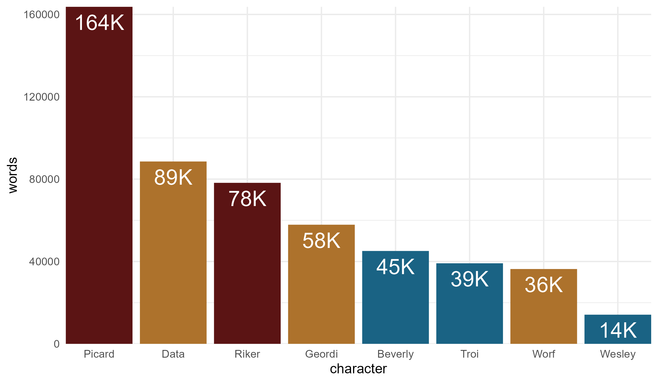
Prominent roles
What is each character’s biggest episode per season in terms of estimated spoken words?
biggest <- filter(x, character %in% id) %>%
  mutate(character = factor(character, levels = id)) %>%
  group_by(season, character) %>%
  summarize(title = title[which.max(words)], words = max(words)) %>%
  arrange(character)

biggest
#> # A tibble: 55 × 4
#> # Groups:   season [7]
#>    season character title                 words
#>     <int> <fct>     <chr>                 <int>
#>  1      1 Picard    Encounter at Farpoint  2575
#>  2      2 Picard    The Measure of a Man   1844
#>  3      3 Picard    The Survivors          1738
#>  4      4 Picard    Devil's Due            2095
#>  5      5 Picard    Ensign Ro              1897
#>  6      6 Picard    The Chase              2083
#>  7      7 Picard    All Good Things...     4019
#>  8      1 Data      Datalore                944
#>  9      2 Data      The Schizoid Man       1592
#> 10      3 Data      The Offspring          1886
#> # ℹ 45 more rows

biggest <- mutate(biggest, winner = character[which.max(words)],
                  ymn = min(words), ymx = max(words)) %>% ungroup() %>%
  mutate(uniform = factor(uniform[match(biggest$character, id)], levels = ulev))

ggplot(biggest, aes(season, words)) +
  geom_linerange(aes(ymin = ymn, ymax = ymx)) +
  geom_point(aes(fill = uniform), shape = 21, size = 2, show.legend = FALSE) +
  scale_fill_manual(values = uniform_colors) +
  geom_text_repel(aes(label = paste0(title, " (", character, ")")),
                  size = 2.3, hjust = -0.1, direction = "y", min.segment.length = 0.65) +
  scale_x_continuous(breaks = 1:7, labels = 1:7, expand = expand_scale(0, c(0.1, 0.8))) +
  theme_minimal(18) + theme(panel.grid.minor = element_blank())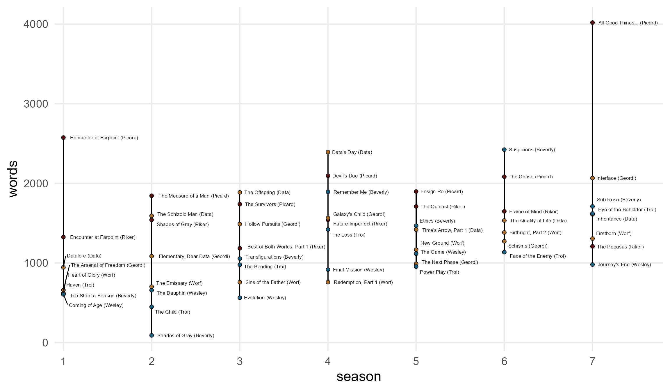
Transferring from TNG to DS9
Finally, look at both Worf and O’Brien, making a comparison between TNG and DS9 in terms of their prominence.
x <- filter(scriptData, format == "episode" & series %in% c("TNG", "DS9")) %>%
  unnest(text) %>%
  select(series, season, title, character, line) %>%
  mutate(character = gsub(pat, "", character)) %>%
  filter(character %in% c("Worf", "O'brien")) %>%
  group_by(series, title, character) %>%
  summarize(lines = n(), words = length(unlist(strsplit(line, " "))))

avg <- group_by(x, series, character) %>%
  summarize(lines = mean(lines), words = mean(words), n_episodes = n()) %>%
  arrange(character, series) %>% ungroup()
avg$character <- gsub("O'brien", "O'Brien", avg$character)

avg
#> # A tibble: 4 × 5
#>   series character lines words n_episodes
#>   <chr>  <chr>     <dbl> <dbl>      <int>
#> 1 DS9    O'Brien    34.5  364.        159
#> 2 TNG    O'Brien    11.6  117.         44
#> 3 DS9    Worf       22.2  227.        100
#> 4 TNG    Worf       24.2  208.        175

id <- rev(unique(avg$character))
chr <- factor(avg$character, levels = id)
avg <- mutate(avg, series = factor(series, levels = c("TNG", "DS9")), character = chr)

ggplot(avg, aes(character, words, fill = series)) +
  geom_col(color = NA, show.legend = FALSE, position = position_dodge()) +
  scale_fill_manual(values = c("dodgerblue", "orange")) +
  geom_text(aes(label = paste0(series, ": ", round(words))),
            size = 10, color = "white", vjust = 1.5,
            position = position_dodge(width = 0.9)) +
  labs(y = "Average words per episode") +
  scale_x_discrete(expand = c(0, 0)) +
  scale_y_continuous(expand = c(0, 0)) +
  theme_minimal(18)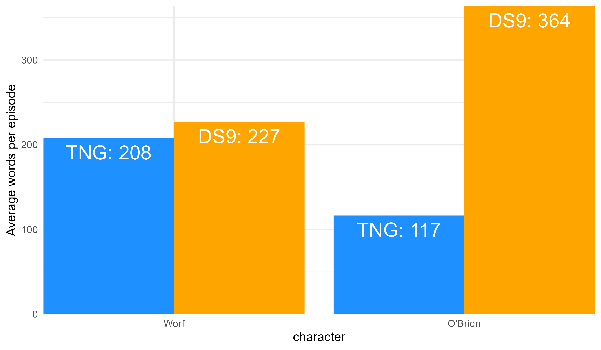
This is a simple exploration of the data, but the results are interesting. Starfleet promotions in rank aside, Worf did not even quite receive a 10% pay bump in terms of average spoken words per episode. On the other hand, O’Brien had an increase of 211%, or more than triple the average number of spoken words per episode when moving from the Enterprise to Deep Space Nine. All things considered, take the transfer. But on spoken words alone, O’Brien was clearly favored. The squeaky wheel gets the grease.
Considerations
This calculation accounts for the number of episodes each character has speaking lines in. For example, TNG episodes missing O’Brien after DS9 began and DS9 episodes missing Worf before he joined the show are not counted against them.
It does not account for episodes where a character may appear in an episode, but without any speaking lines, which should drop their averages. However, this is rare and, if anything, I would expect it to exacerbate the difference seen here rather than diminish it. I’m just guessing there may have been some early TNG episodes where O’Brien was shown but never spoke.
A more rigorous approach that I may show in a subsequent example would be to join this transcript data with episode casting data from STAPI so that there is no need to rely on speaking lines in transcripts to guess at whether someone was featured in an episode.