The tabr tutorials began with a basic example that
introduced the general workflow.
- Define a musical phrase with
phrase()or the shorthand aliasp(). - Add the phrase to a
track(). - Add the track to a
score(). - Render the score to pdf with
tab()or anotherrender_*function.
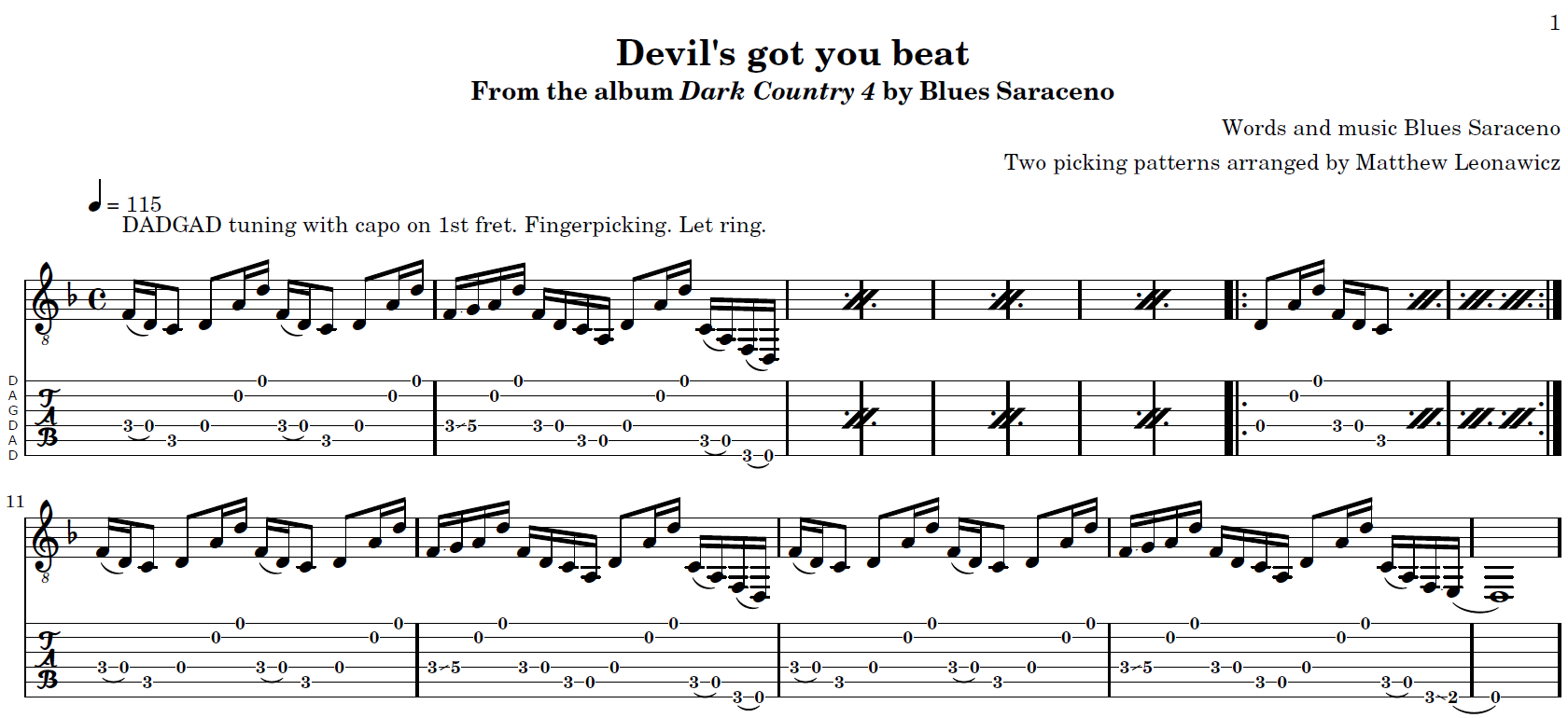
This short R script example is more complex. It does not represent a complete tab of a song; it is just a short arrangement of two basic fingerpicking patterns similar to but not exactly the same as heard in Blues Saraceno’s Devil’s got you beat. The second pattern is actually just a small slice of the first pattern that is shifted in time slightly. While not a complete tab, it is much more thorough than the opening tutorial example, making use of several techniques and functions that have been covered.
Some of the most interesting things to note below include:
- Non-standard tuning (DADGAD) plus a capo on the first fret.
- Use of all the available song information arguments in
header. - Nested repeats with percent repeats applied inside of a volta repeat.
- Avoidance of repetition of the text annotation attached to the opening note when using percent repeats.
R code
header <- list(
  title = "Devil's got you beat",
  composer = "Words and music Blues Saraceno",
  performer = "Blues Saraceno",
  album = "Dark Country 4",
  subtitle = "From the album Dark Country 4 by Blues Saraceno",
  arranger = "Two picking patterns arranged by Matthew Leonawicz",
  copyright = "2016 Extreme Music"
)

txt <- c("DADGAD tuning with capo on 1st fret. Fingerpicking. Let ring.")
tuning <- "d, a, d g a d'"

# melody 1
notes <- c(pn("f d c d a d'", 2), "f g a d' f d c a,")
info <- purrr::map_chr(c("16(", notate("16(", txt)),
                       ~pc(.x, "16) 8 8 16 16 16( 16) 8 8 16 16 16- 16*7"))
strings <- "4 4 5 4 2 1 4 4 5 4 2 1 4 4 2 1 4 4 5 5"
p1 <-purrr::map(info, ~p(notes, .x, strings))
e1 <- p("d a d' c a, f, d,", "8 16 16 16( 16) 16( 16)", "4 2 1 5 5 6 6")
e2 <- p("d a d' c a, f, e, d,", "8 16 16 16( 16) 16- 16( 1)", "4 2 1 5 5 6 6 6")

#melody 2
p2 <- p("d a d' f d c", "8 16*4 8", "4 2 1 4 4 5")

p_all <- c(pct(c(p1[[2]], e1), 3), volta(pct(p2, 3), 1), p1[[1]], e1, p1[[1]], e2)
track(p_all, tuning = tuning) |> score() |>
  tab("out.pdf", "dm", "4/4", "4 = 115", header)
You can see above that notate() can often obstruct
otherwise convenient opportunities for code reduction. Avoiding
repeating the annotation means avoiding repeating whatever it is bound
to. This is not a problem for percent repeats because there is nothing
to show, but would be for the repetitions of the melody at the end of
the score. This is why info was mapped to a length 2 vector
using an opening note with and without a bound text annotation,
respectively.
The e1 and e2 endings on the phrase
p1 were not used as default and alternate endings in a call
to volta(), respectively, because they would fail the bar
check; p1 alone does not end at the end of a measure, but
rather lasts for a measure and a half. This example also shows how a
single note difference at the very end of the second ending,
e2, an ending that is only played once at the end of the
arrangement, is enough to stop you from defining what would sensibly be
the full phrase (p1 through e1) as such. The
slightest change forces you to split things up and expand the code, just
like in a tab. And most music, at least the kind for which there is any
point in transcribing, is going to change things up often even for
repeated sections.
Result
The result of the call to tab() is as follows.
The next example refactors the phrases above to properly represent multiple voices in the output.