Data Extraction Evaluation
Matthew Leonawicz
Results
All points? No point.
Using the sample mean is helpful as a data reduction strategy while not being harmful in terms of representativeness. The possible “tradeoff” itself appears to be largely a false dichotomy. There is no benefit to computing the mean of all pixels in the example map layer.
How many samples do we really need?
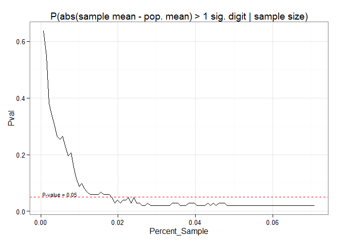
In this example even a two percent subsample of the original non-NA data cells is small enough to limit us to a five percent probability of obtaining a mean that differs from the mean computed on the full dataset by an amount equal to or greater than the smallest discrete increment possible (0.1 degrees Celsius for SNAP temperature data) based simply on the number of significant figures present. Furthermore, even for nominal sample sizes, the 0.05 probability is one almost strictly of minimal deviation (0.1 degrees). The probability that a sample mean computed on a subsample of the map layer deviates enough from the population mean to cause it to be rounded to two discrete incremental units from the population mean (0.2 degrees) is essentially zero (except if using crudely small sample sizes).
Although a two percent subsample appears sufficient for this criterion, let’s use a five percent subsample for illustration. This is clearly overkill in this example since the p-value attenuates to the range of 0.019 to 0.029 by around 2.5 percent subsampling.
How much faster does this make things go?
Compute time for the mean is of course affected by the sample size.
## Unit: microseconds
##                          expr    min     lq      mean median     uq
##  sum(s005pct)/length(s005pct)  4.665  4.977  5.131030  4.977  4.977
##  sum(s010pct)/length(s010pct)  9.330  9.331  9.735872  9.642  9.642
##  sum(s025pct)/length(s025pct) 23.015 23.016 23.542057 23.326 23.327
##  sum(s100pct)/length(s100pct) 91.435 91.747 92.423067 91.747 91.747
##      max neval
##  103.565 10000
##  127.201 10000
##  137.153 10000
##  440.693 10000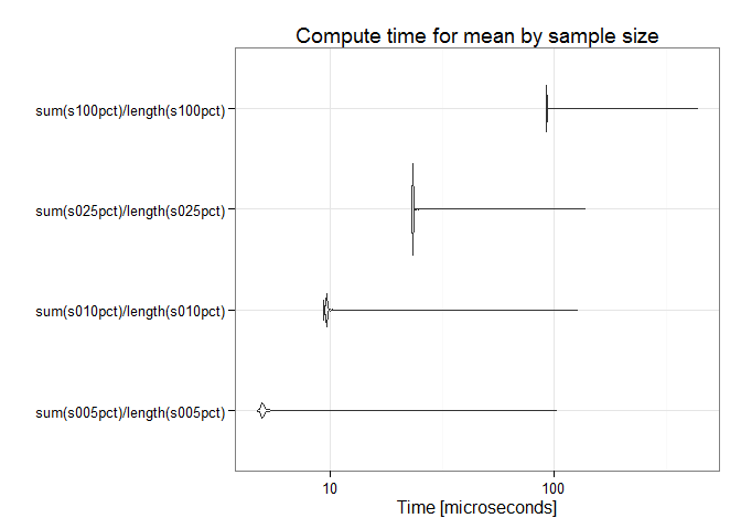
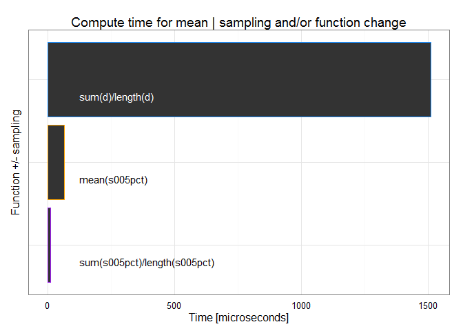
Using optimal subsampling to estimate the mean achieves speed improvements orders of magnitude greater than what can be achieved through strictly algorithmic changes to how the mean is computed on the full dataset, though those help immensely as well, also by many orders of magnitude. Sampling is vastly more effective, but both approaches can be combined for maximum benefit.
## Unit: microseconds
##                          expr        min         lq         mean
##  sum(s005pct)/length(s005pct)      4.977      6.843      9.85981
##            mean(v, na.rm = T) 328144.555 330528.395 336360.45702
##              sum(d)/length(d)   1493.750   1504.635   1529.18558
##                 mean(s005pct)     19.283     22.705     52.17487
##      median          uq        max neval
##       9.953     11.1970     17.106   100
##  331091.000 340133.4210 431130.188   100
##    1510.544   1539.7785   1683.461   100
##      65.933     70.4435     94.857   100
## Unit: microseconds
## expr min lq mean
## sum(s005pct)/length(s005pct) 4.977 6.843 9.85981
## mean(v, na.rm = T) 328144.555 330528.395 336360.45702
## sum(d)/length(d) 1493.750 1504.635 1529.18558
## mean(s005pct) 19.283 22.705 52.17487
## median uq max neval
## 9.953 11.1970 17.106 100
## 331091.000 340133.4210 431130.188 100
## 1510.544 1539.7785 1683.461 100
## 65.933 70.4435 94.857 100## Unit: microseconds
## expr min lq mean
## sum(s005pct)/length(s005pct) 4.977 6.843 9.85981
## mean(v, na.rm = T) 328144.555 330528.395 336360.45702
## sum(d)/length(d) 1493.750 1504.635 1529.18558
## mean(s005pct) 19.283 22.705 52.17487
## median uq max neval
## 9.953 11.1970 17.106 100
## 331091.000 340133.4210 431130.188 100
## 1510.544 1539.7785 1683.461 100
## 65.933 70.4435 94.857 100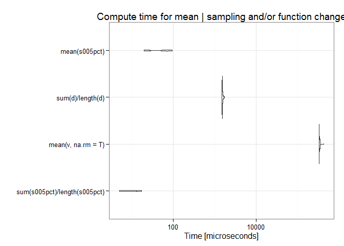
Similar to above, below are the median compute times for the mean using (1) the full data while removing NAs, (2) the sum divided by the length after NAs removed, (3) the mean of a subsample, and (4) a combination of (2) and (3).
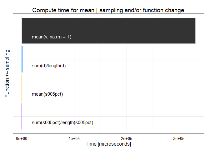
Here is the same plot after removing the first bar to better show the relative compute time for the other three methods.
How does the benefit extend to extractions on maps at different extents, data heterogeneity, climate variables, or for other common statistics such as the standard deviation? These are open questions at the moment, but for one thing, I expect more samples are needed for precipitation than temperature. I also expect more samples needed to estimate parameters with higher moments.