Data Extraction Evaluation
Matthew Leonawicz
Next steps
Combining sampling and data reduction methods while using the most efficient R functions can be particularly useful when processing large numbers of high-resolution geotiff raster layers. One thing I already do when extracting from many files by shapefile is I avoid extracting by shape more than once. I do it one time to obtain the corresponding raster layer cell indices. Then on all subsequent maps I extract by cell indices which is notably faster. Ultimately, there is much more room for speed improvements in terms of efficient use of statistics than in strictly programmatic corner-cutting.
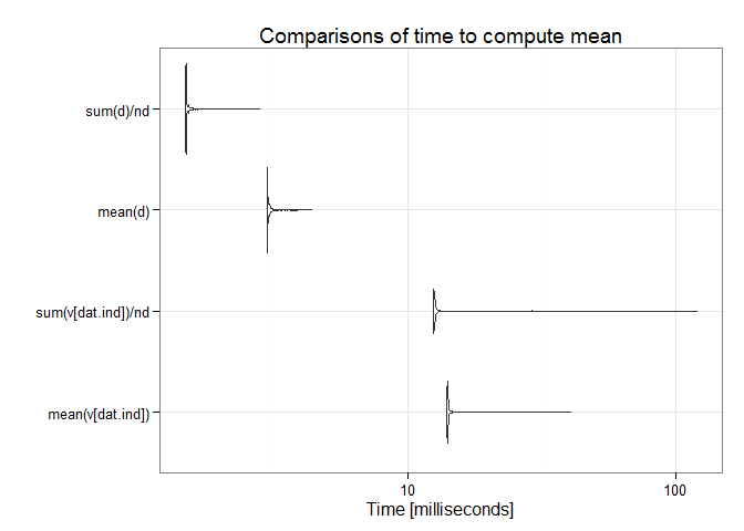
The plots below benchmark different sample mean computations. Comparisons involve the sample mean of the entire data set and do not involve the main approach outlined above which focuses on efficiency gains by taking the mean of a smaller, representative sample. This provides some insight into how it is beneficial nonetheless to considering the right programmatic approach in conjunction with statistical efficiencies.
## Unit: milliseconds
##                              expr       min        lq      mean    median
##                mean(v, na.rm = T) 329.44610 330.05676 335.42389 330.57520
##                  mean(v[dat.ind])  13.95565  14.04958  15.29547  14.12624
##                sum(v[dat.ind])/nd  12.42334  12.51275  14.71309  12.59486
##       .Internal(mean(v[dat.ind]))  13.87759  13.97556  16.08770  14.05844
##  .Primitive("sum")(v[dat.ind])/nd  12.41090  12.51306  14.51659  12.59221
##         uq       max neval
##  333.69472 436.24961   100
##   14.20492  36.44741   100
##   12.70713  35.46495   100
##   14.18844  39.18424   100
##   12.69065  36.18741   100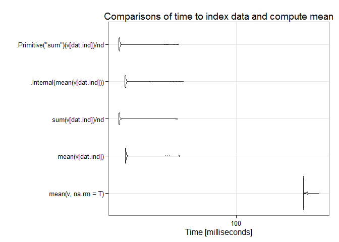
## Unit: milliseconds
##                expr       min        lq      mean    median        uq
##    mean(v[dat.ind]) 13.940724 14.054862 15.692511 14.112709 14.212696
##  sum(v[dat.ind])/nd 12.418051 12.527058 14.080500 12.576819 12.663589
##             mean(d)  2.999005  3.010046  3.048648  3.018910  3.047055
##           sum(d)/nd  1.495927  1.500281  1.526706  1.504635  1.514277
##         max neval
##   40.684519  1000
##  120.171675  1000
##    4.425889  1000
##    2.837906  1000