Downscaling minimum, mean and maximum temperatures

Independent application of the delta method. What can go wrong?

When downscaling monthly averages of global climate model minimum, mean and maximum temperature outputs to a high-resolution climatology it is possible for the downscaled outputs to lose the property of monotonically increasing minimum to mean to maximum temperatures. This is a serious violation of the support of the multivariate temperature distribution. While this is not guaranteed to happen, it is also not prohibited from happening when using the univariate delta downscaling.

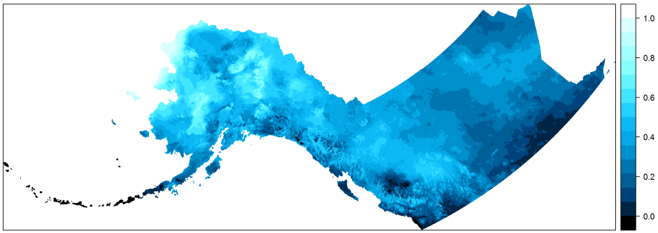
A spatially explicit view of the proportion of years in a 95-year projected period during which downscaled minimum temperatures exceed mean temperatures for a particularly problematic combination of GCM and PRISM climatologies. In many locations the violation occurs every year.

For clarity, note that when I refer to minimum, mean and maximum temperatures, this is shorthand for the monthly means of the daily minimum, mean and maximum temperatures, respectively.

Other methods might be more robust to this violation in cases where it would happen with the delta method, but if another downscaling method is also univariate and applied independently to the variables, at a minimum it is not readily clear how or why the same issue would be prohibited from happening.

This method can be applied separately and independently to each of these three ordered temperature variables. Intuitively, it is easy to understand that, for example, when downscaling mean monthly minimum temperature, the procedure has no awareness that there is another downscaled data set of mean temperatures which it cannot exceed. Similarly, when downscaling maximum temperature, nothing stops a downscaled value from dipping below the mean, or even the minimum.

Values of the three variables may go out of order for a given grid cell and time point. This can occur due to differences between a GCM and a chosen climatology data set in terms of the intra-day temperature variability on which their respective monthly averages are based.

A GCM might reveal a relatively large gap between minimum and maximum temperature in a region. This gap may shrink over time as the minimum temperature increases with time more than the maximum increases. This difference in deltas between two time points is of course restricted in the GCM to how much separation were initially between the minimum and maximum. However, high-resolution minimum and maximum temperature climatology data sets utilized for downscaling these variables may not accommodate such a gap.

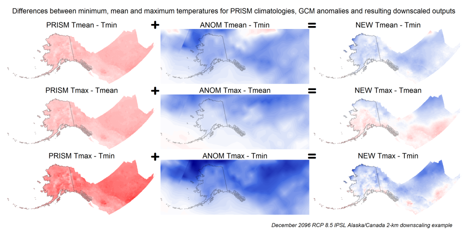
Gaps between minimum, mean and maximum temperatures are shown (vertically) as difference maps. Each row shows how when interpolated anomalies are added to the high-resolution PRISM climatologies, the differences in anomalies may combine with the differences in PRISM climatologies to allow for regions of out of order temperature statistics. Red highlights anything positive and blue negative. Note that negative values are fine in the middle column because, for example, a minimum temperature anomaly may be greater than a maximum temperature anomaly. However, the differences in downscaled outputs shown in the third column should be all non-negative, like they are in the first column.

As an example, say a GCM minimum temperature climatology is 2 degrees C in a given area and the maximum temperature climatology is 8 degrees. At some point in the future, both variables have increased in temperature over time, but by different amounts. The minimum temperature has gone up more in the future than maximum temperature, which is not unusual. The values have increased from 2 and 8 to 9 and 12, respectively.

That gives us anomalies, or deltas, of 7 degrees for minimum temperature and 4 degrees for maximum temperature. These values are added onto new minimum and maximum temperature climatologies during the downscaling process. However, the minimum and maximum temperature climatology values in this area, instead of being 2 and 8 degrees C like in the original GCM climatology, are 3 and 5 degrees C. When the anomalies of 7 and 4 are added to these values, the resulting downscaled minimum and maximum temperatures are now 10 and 9 degrees C, respectively.

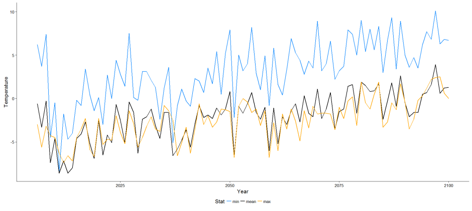
Time series of downscaled outputs for a grid cell where at least one violation occurs every year.

Conditional delta downscaling

This is an inherent limitation of the univariate deltas method. It may not occur at all when downscaling multiple ordered variables, but with the right combination of climate model output and choice of climatology, this is an expected outcome. Clearly, order statistics which do not behave and which may change their ordering do not belong in this universe. Something must be done to maintain a valid support for the multivariate temperature distribution.

The violation of the requirement that the minimum, mean, and maximum be in proper ascending order may occur when attempting to downscale these three climate variables to three different climatologies. While the original GCM variables and the high-resolution climatologies each have a valid support for their multivariate temperature distribution, the GCM and the data set to which it is being downscaled may be sufficiently different from each other to invalidate the new support.

Instead of independently downscaling all three variables the the three high-resolution climatologies, a chain method for delta downscaling is used. First, mean temperature is downscaled to the high-resolution mean temperature climatology. Second, minimum and maximum temperatures are downscaled with respect to the previously downscaled mean temperature.

This reduces the dimensionality of the problem. It can be viewed as removing degrees of freedom. However you wish to look at it, the key change is making the downscaling of these three ordered variables dependent on one high-resolution climatology rather than three. Downscaling is no longer done independently for the three temperature data sets. The GCM mean temperature outputs are downscaled to a mean temperature climatology. In our case we use the PRISM mean temperature climatology for Alaska and western Canada. The GCM minimum and maximum temperatures are transformed into new random variables, which are functions of mean temperature and are then each downscaled conditional on the downscaled mean temperature data.

GCM mean temperature is downscaled to the PRISM 1961-1990 mean temperature climatology using the delta method without any changes. The general algorithm for conditional delta downscaling, the second round of downscaling in the chain method, is as follows:

Using the raw GCM data, for each grid cell and time point compute the random variables X = minimum temperature - mean temperature and Y = maximum temperature - mean temperature.

If you imagine the GCM data as stacks of temperature maps through time, we now have two stacks of temperature difference maps, or “gap maps” through time. These are our anomalies, or deltas. The difference from the usual delta downscaling method is that in this application of conditional delta downscaling the deltas map layer for a given time slice contains deltas with respect to mean temperature at that same time slice rather than deltas with respect to the same variable (minimum or maximum temperature) from a different time slice (or rather, a climatology). We are working with the deviations above and below the mean temperature defining the maximum and minimum temperatures.

Interpolate the deltas to our 2-km PRISM resolution, as would normally be done with delta layers in delta downscaling.
Add the temperature delta map layers X and Y onto downscaled mean temperature instead of onto minimum and maximum temperature PRISM climatologies; these climatologies are not used.

This essentially is delta downscaling, only reframed in a perspective that accounts for the relationship of minimum and maximum temperatures to mean temperature - or rather, the relationship of the mean to the minimum and maximum since in climate model outputs the mean may have been derived secondarily, estimated as the midrange of the minimum and maximum temperature outputs.

Performing delta downscaling using the chain method, with conditional delta downscaling of minimum and maximum temperature-defining deviations from the mean being downscaled to the initially downscaled mean temperature. This yields a multivariate temperature distribution with a valid support where the minimum, mean and maximum temperatures are properly ordered.

Here is a comparison of the methods using the time series for a given grid cell.

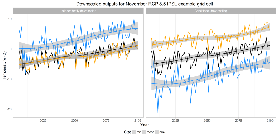
When the ordered temperature variables are downscaled to the respective PRISM climatologies, order is not preserved. Order is preserved with conditional delta downscaling because the relationships of minimum and maximum temperature to mean temperature in the raw GCM data are maintained via the dependency chain.

Some points to note about this approach

Conditional delta downscaling of minimum and maximum temperature on downscaled mean temperature directly addresses the order statistics violation where monotonically increasing minimum, mean and maximum temperatures are required, given that proper order is observed in the raw GCM data.
Procedurally, the conditional delta downscaling method is a clear analog to the initial, usual delta downscaling method.
This method leaves mean temperature alone, allowing it to be downscaled in the standard manner.
The downscaled outputs retain information about separation of minimum and maximum from mean in both time and space that was present in the raw GCM inputs.
No complex statistical model is required to be coupled the delta method to address the multivariate support violation. The same basic delta method concepts are applied as a chain method; only the reference used to describe the deltas changes - mean temperature with respect to the PRISM climatology and then minimum and maximum temperatures with respect to mean temperature.
Unlike direct downscaling to PRISM where independent application of the delta method to all three variables was at the root of the problem, minimum and maximum temperature can be treated independently because it is actually their differences from the mean which are downscaled. These transformed random variables are both functions of mean temperature and are both downscaled to the same 2-km mean temperature data set.
It would not be sufficient to downscaled minimum and maximum GCM temperatures to PRISM minimum and maximum temperature climatologies and then define downscaled mean temperature as the midpoint of the other two downscaled data sets. This merely reduces the number of independently downscaled ordered temperature variables to unique PRISM temperature climatologies from three to two. While this would force the mean to always be between the minimum and the maximum, the order statistics violations remain present in the outputs; minimum and maximum temperatures may still reverse order.

R code for conditional delta downscaling

Setup

This is not all necessary, but it may be more convenient to run in non-interactive mode via Rscript. We load required packages and set up some input and output directories.

if (interactive()) {
    gcm <- "IPSL-CM5A-LR"
    rcp <- "rcp85"
} else {
    comargs <- (commandArgs(TRUE))
    if (length(comargs)) 
        for (z in 1:length(comargs)) eval(parse(text = comargs[[z]]))
    if (!exists("rcp") | !exists("gcm")) 
        stop("Must provide valid 'rcp' and 'gcm' args.")
}

library(parallel)
library(rgdal)
library(raster)
library(purrr)
rasterOptions(chunksize = 1e+11, maxmemory = 1e+12)

setwd("/workspace/Shared/Tech_Projects/EPSCoR_Southcentral/project_data")
rawDir <- "cmip5/prepped"
dsDir <- "downscaled"
vars <- c("tasmin", "tas", "tasmax")
dir.create(outDir <- file.path("/atlas_scratch/mfleonawicz/tas_minmax_ds", gcm, 
    rcp), recur = T, showWarnings = F)
walk(vars[c(1, 3)], ~dir.create(file.path(outDir, .x), showWarnings = F))

Functions

There are only a few functions here and they are all very simple. devFromMean uses the raster package to interface with netcdf, reading the minimum, mean and maximum temperature files into bricks for a given RCP and GCM. It returns a list of the two desired bricks of deltas.

fortify prepares raw GCM raster layers for projection to the higher-resolution grid. This may not be necessary depending on the GCM data. dsFiles simply returns a list of files names for the corresponding downscaled mean temperature single-layer geotiff outputs. In my case the files need some reordering to line up with the chronological raw GCM brick layers due to a silly file naming convention, so that part can possibly be ignored as well.

Finally, writeMinMax is the function which performs the basic delta arithmetic operations and writes conditionally downscaled minimum and maximum temperature map layer geotiffs to disk.

devFromMean <- function(rcp, gcm) {
    if (gcm == "NCAR-CCSM4") 
        gcm <- "CCSM4"  # temporary fix: raw files have different name
    x <- map(vars, ~readAll(brick(list.files(file.path(rawDir, gcm, rcp, .x), 
        full = T), varname = .x)))
    list(lwr = x[[1]] - x[[2]], upr = x[[3]] - x[[2]])
}

fortify <- function(x) {
    r <- raster(extent(0, 360, -90, 90), nrow = nrow(x), ncol = ncol(x), crs = projection(x))
    round(rotate(resample(x, r)), 1)
}

dsFiles <- function(rcp, gcm) {
    v <- list.files(file.path(dsDir, gcm, rcp, vars[2]), full = T)
    yrs <- as.integer(substr(map_chr(strsplit(basename(v), "_"), 8), 1, 4))
    v <- as.character(unlist(split(v, yrs)))
    list(gsub(vars[2], vars[1], v), v, gsub(vars[2], vars[3], v)) %>% setNames(vars)
}

writeMinMax <- function(i, x, y, dir) {
    r <- readAll(raster(y$tas[i]))
    rmin <- round(r + projectRaster(subset(x$lwr, i), r), 1)
    rmax <- round(r + projectRaster(subset(x$upr, i), r), 1)
    walk2(list(rmin, rmax), vars[c(1, 3)], ~writeRaster(.x, file.path(outDir, 
        .y, basename(y[[.y]][i])), datatype = "FLT4S", overwrite = T))
    print(paste("File", i, "of", length(y$tas), "saved."))
}

Downscale

Compute raw GCM deviations from mean and list corresponding downscaled mean files. Pass both to writeMinMax and run in parallel across time.

deltas <- devFromMean(rcp, gcm) %>% map(~fortify(.x))
files <- dsFiles(rcp, gcm)
mclapply(seq_along(files$tas), writeMinMax, deltas, files, mc.cores = 32)